Approximating Palettes from Other Packages
approximations.RmdOverview
The flexible specification of HCL-based color palettes in colorspace allows one to closely approximate color palettes from various other packages:
- ColorBrewer.org (Harrower and Brewer 2003) as provided by the R package RColorBrewer (Neuwirth 2014).
- CARTO colors (CARTO 2019) as provided by the R package rcartocolor (Nowosad 2019).
- The viridis palettes of Smith and Van der Walt (2015) developed for matplotlib, as provided by the R package viridis (Garnier 2018).
- The scientific color maps of Crameri (2018) as provided by the R package scico (Pedersen and Crameri 2020).
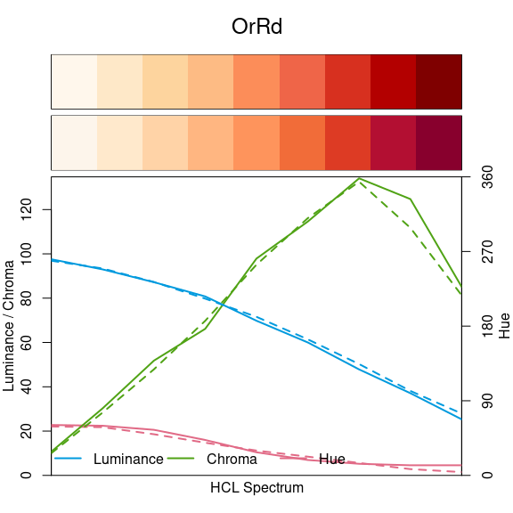
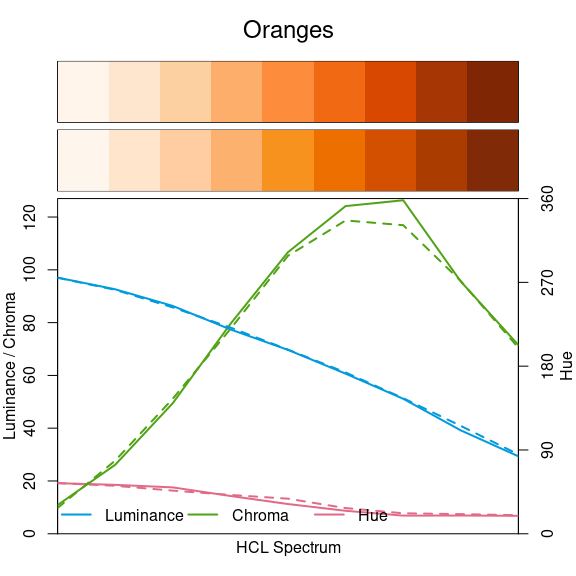
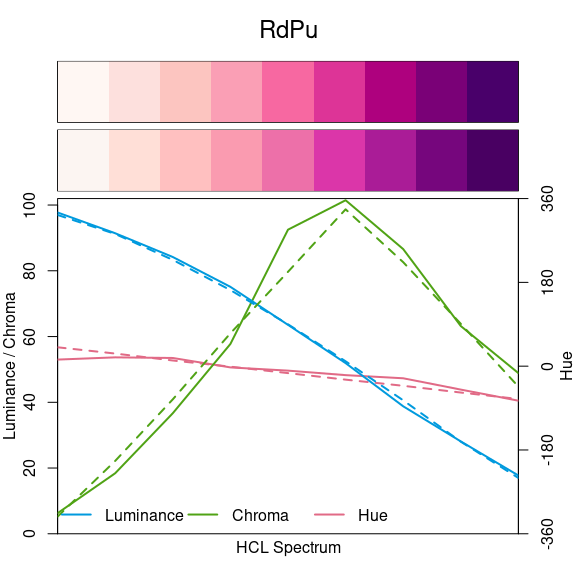
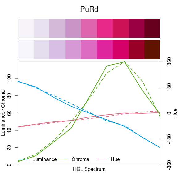
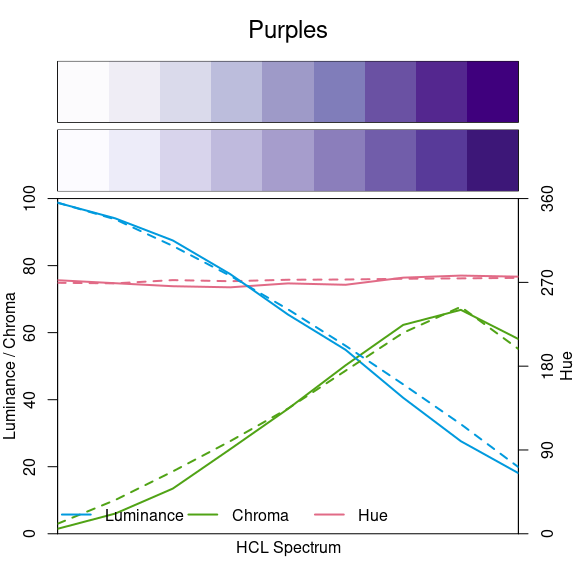
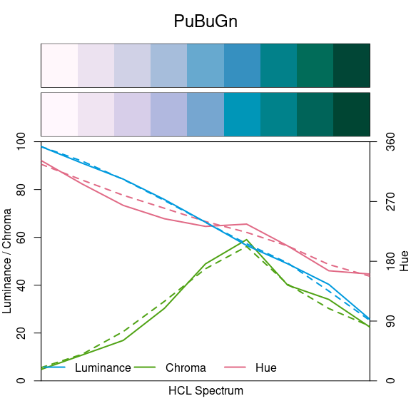
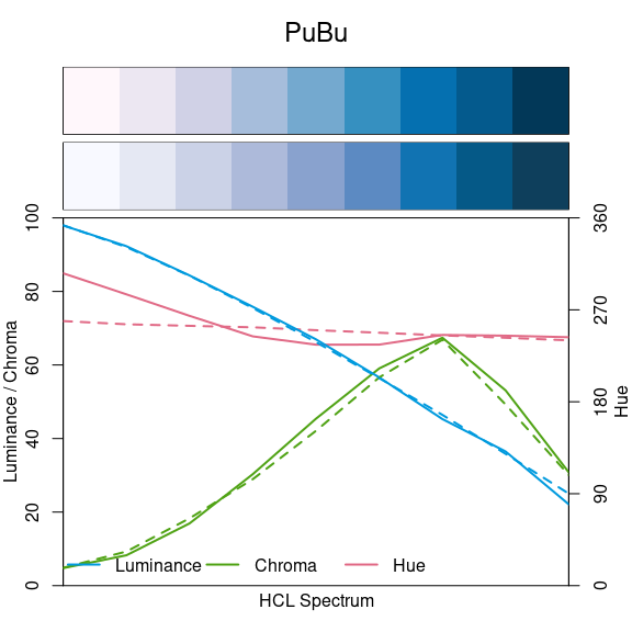
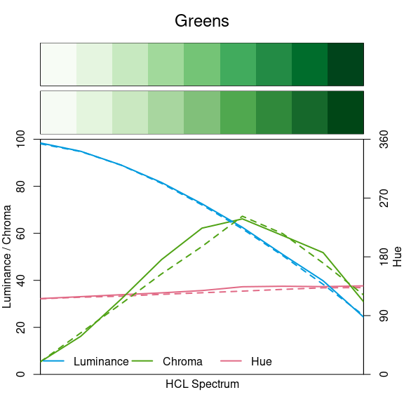
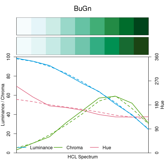
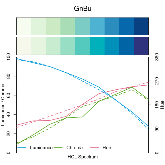
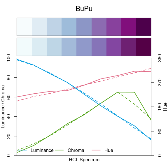
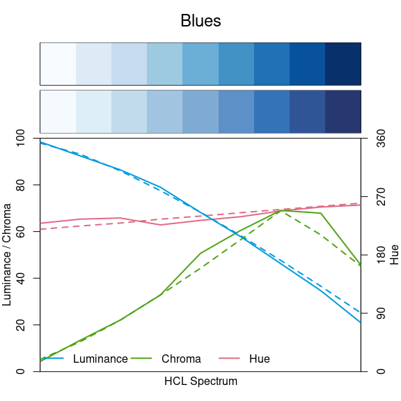
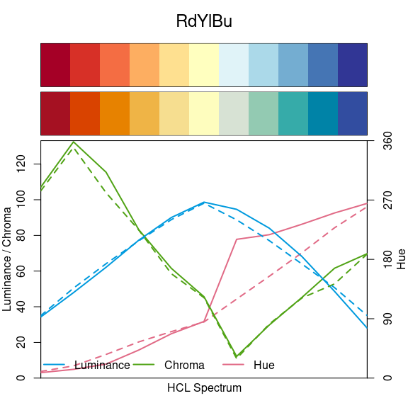
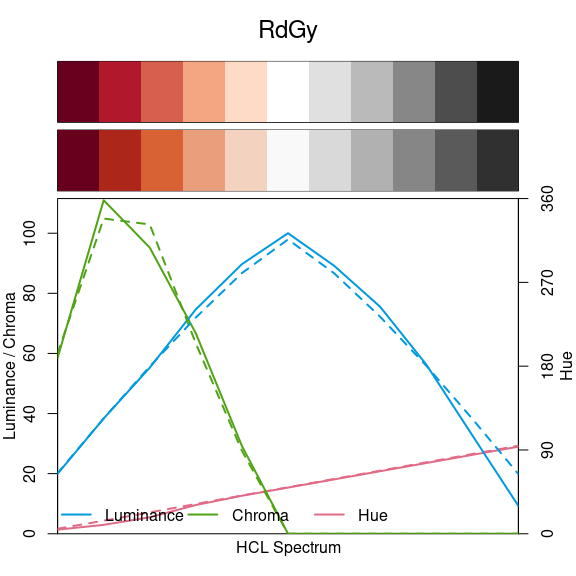
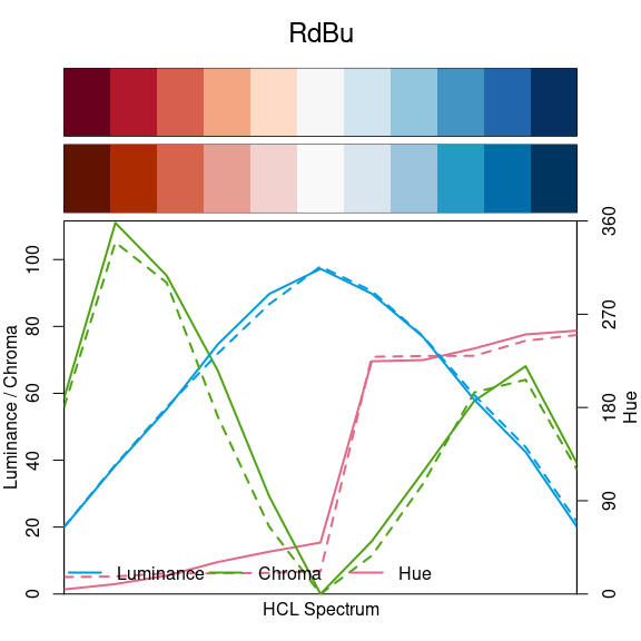
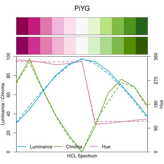
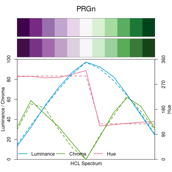
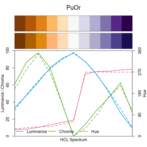
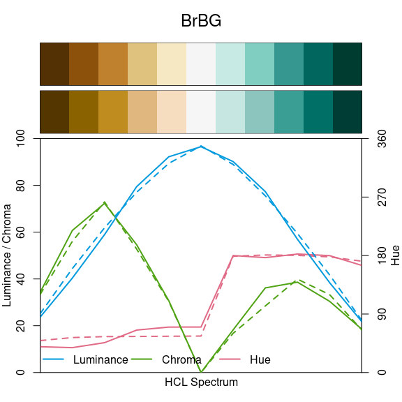
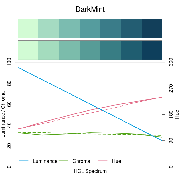
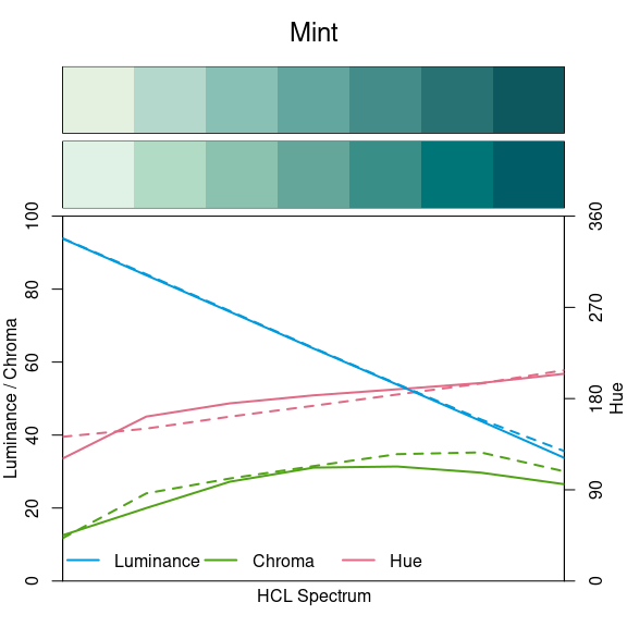
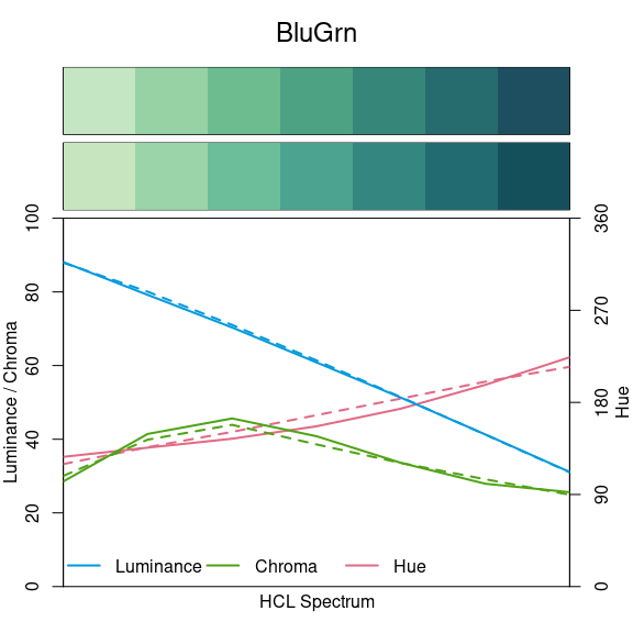
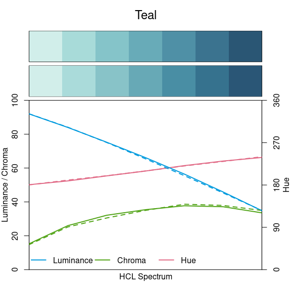
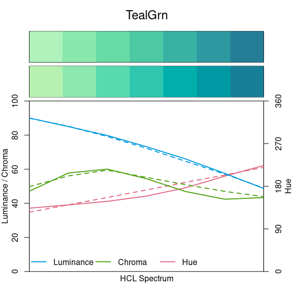
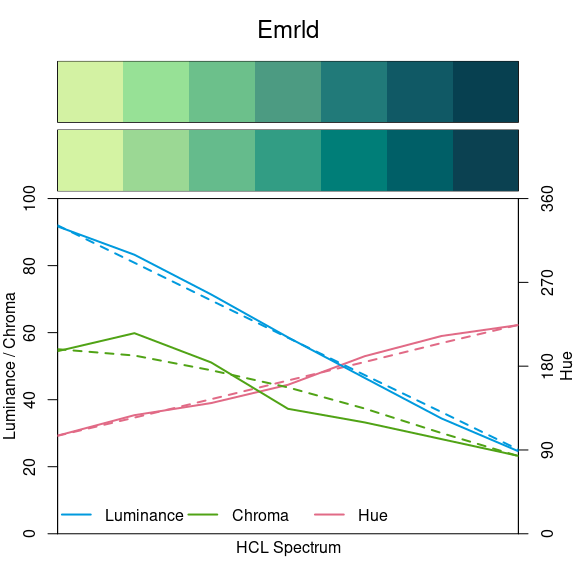
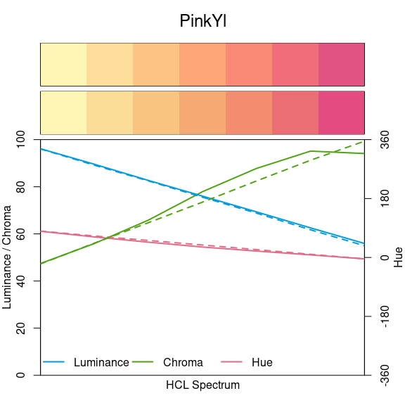
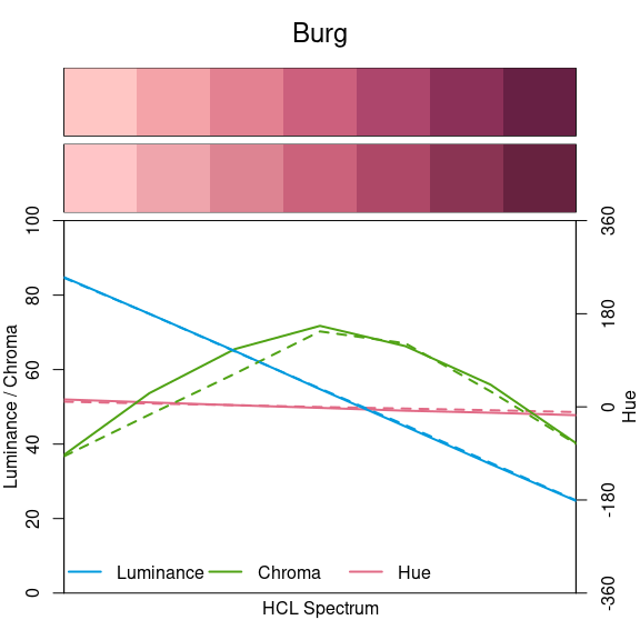
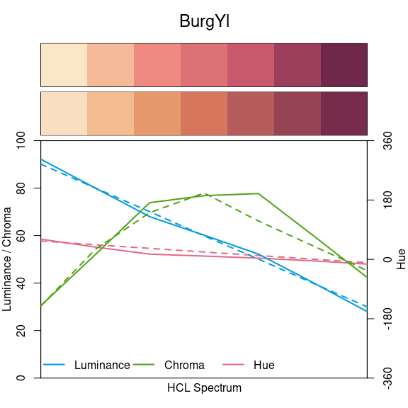
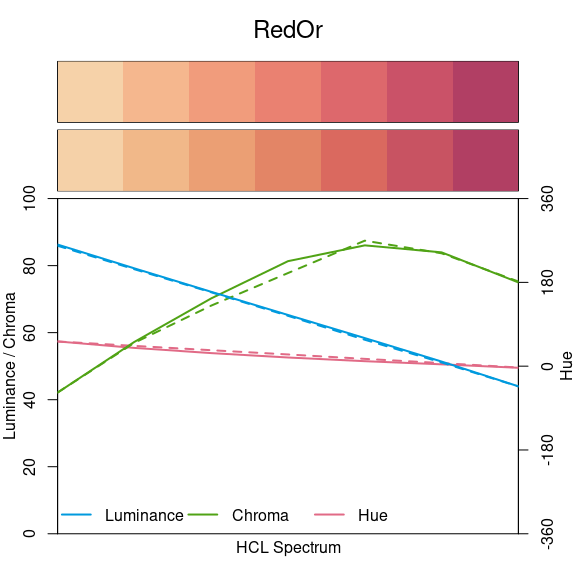
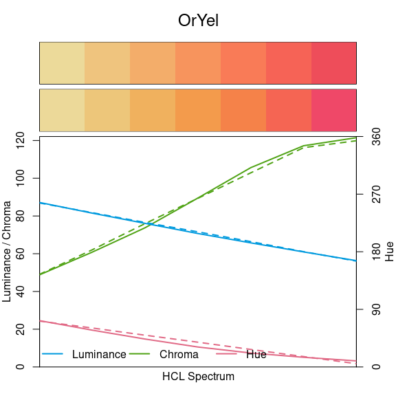
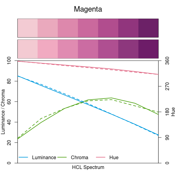
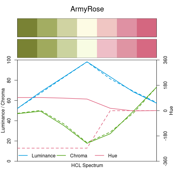
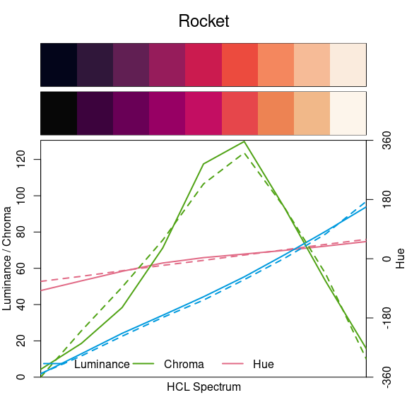
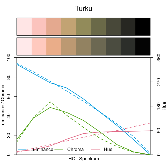
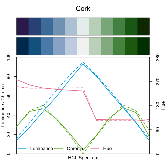
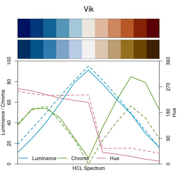
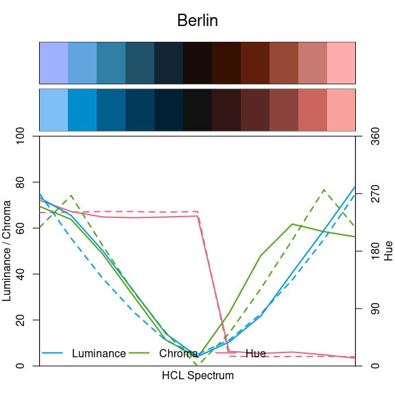
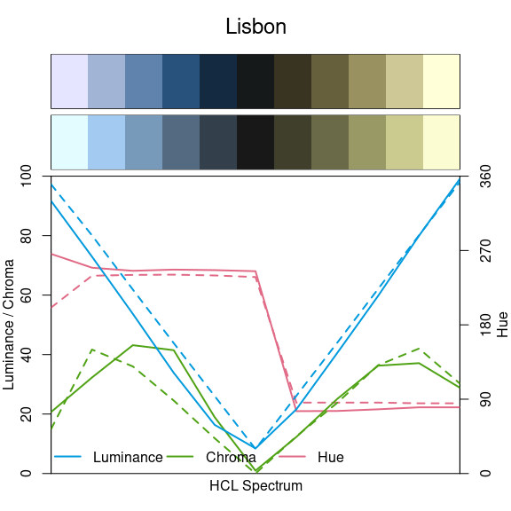
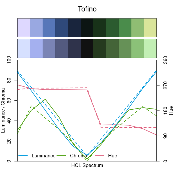
See the discussion of HCL-based
palettes for more details. In the following sections
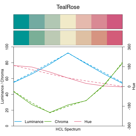
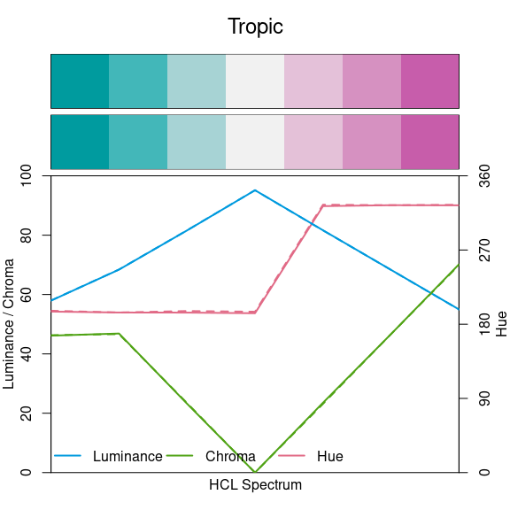
specplot() is used to compare the HCL spectrum
of the original palettes (top swatches, solid lines) and their HCL-based
approximations (bottom swatches, dashed lines).
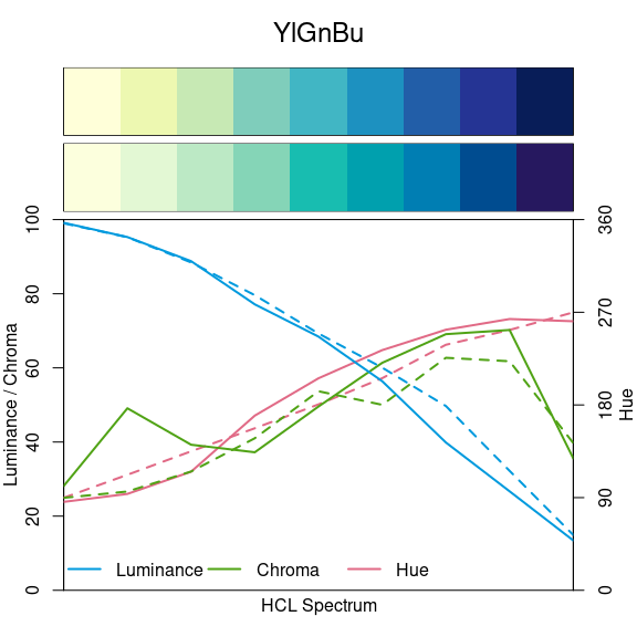
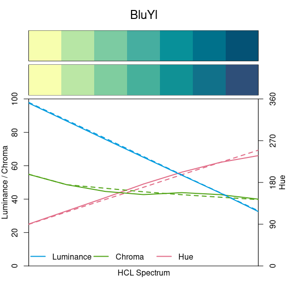
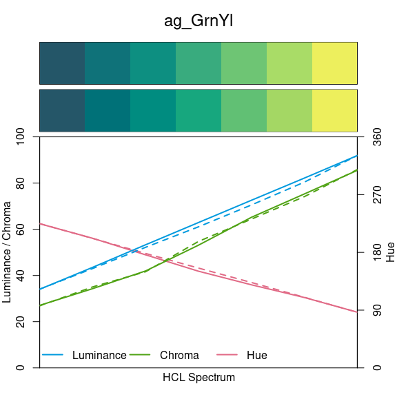
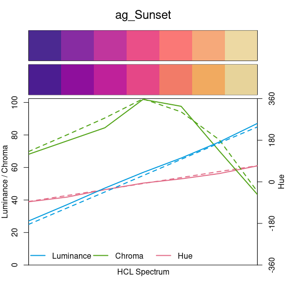
Before, a selection of such approximations using
specplot() is highlighted and discussed in some more
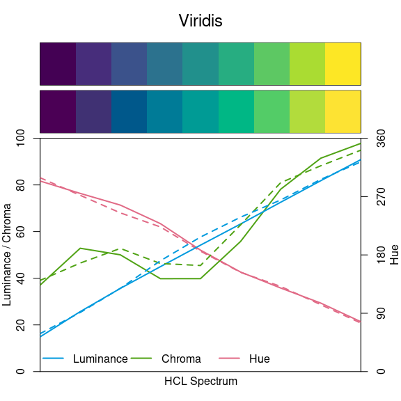
detail. Specifically, the graphic below shows two blue/green/yellow
palettes (RColorBrewer::brewer.pal(7, "YlGnBu") and
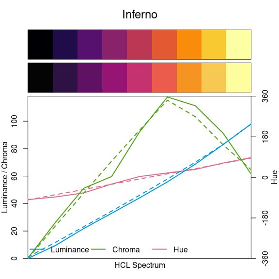
viridis::viridis(7)) and two purple/red/yellow palettes
(rcartocolor::carto_pal(7, "ag_Sunset") and
viridis::plasma(7)). Each panel compares the hue, chroma,
and luminance trajectories of the original palettes (top swatches, solid
lines) and their HCL-based approximations (bottom swatches, dashed
lines). The palettes are not identical but very close for most colors.
Note also that the chroma trajectories from the HCL palettes (green
dashed lines) have some kinks which are due to fixing HCL coordinates at
the boundaries of admissible RGB colors.
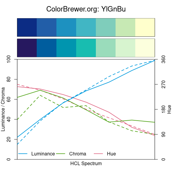
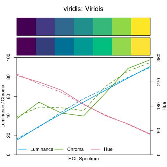

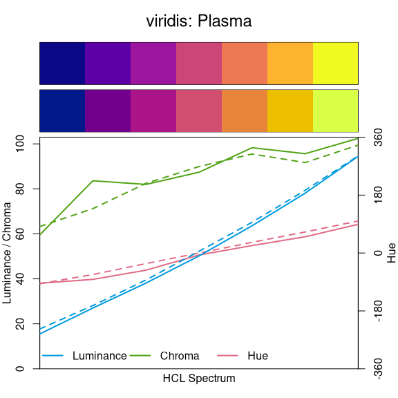
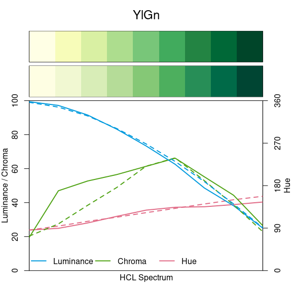
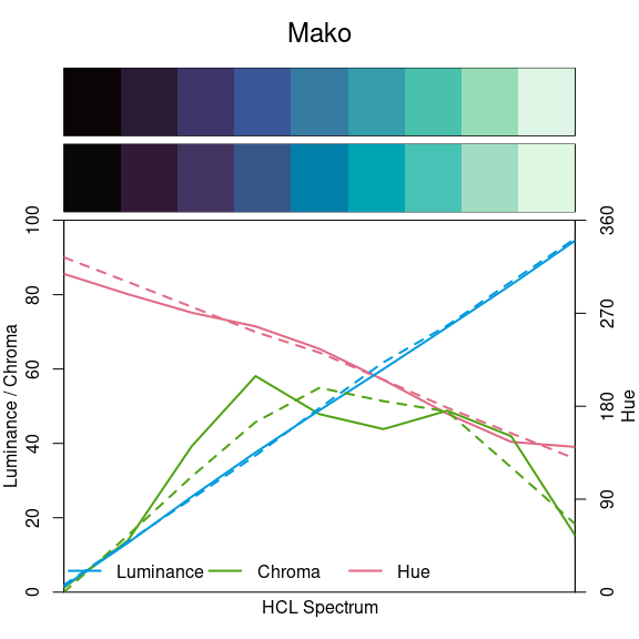
These graphics illustrate what sets the viridis palettes apart from
other sequential palettes. While the hue and luminance trajectories of
"Viridis" and "YlGnBu" are very similar, the
chroma trajectories differ: While lighter colors (with high luminance)
have low chroma for "YlGnBu", they have increasing chroma
for "Viridis". Similarly, "ag_Sunset" and
"Plasma" have similar hue and luminance trajectories but
different chroma trajectories. The result is that the viridis palettes
have rather high chroma throughout which does not work as well for
sequential palettes on a white/light background as all shaded areas
convey high “intensity”. However, they work better on a dark/black
background. Also, they might be a reasonable alternative for qualitative
palettes when grayscale printing should also work.
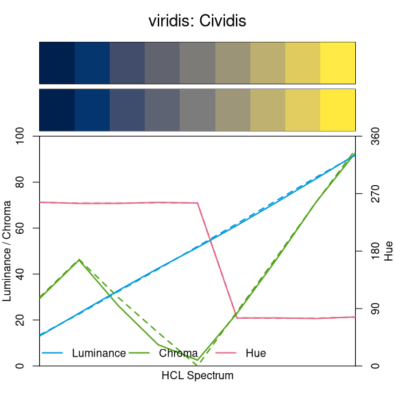
Another somewhat nonstandard palette from the viridis family is the
cividis palette based on blue and yellow hues and hence safe for
red-green deficient viewers. The figure below shows the corresponding
specplot() along with an HCL-based approximation. This
palette is unusual: The hue and chroma trajectories would suggest a
diverging palette, as there are two “arms” with different hues and a
zero-chroma point in the center. However, the luminance trajectory
clearly indicates a sequential palette as colors go monotonically from
dark to light. Due to this unusual mixture the palette cannot be
composed using the trajectories discussed in the construction
details.
However, the tools in colorspace can still be employed to easily reconstruct the palette. One strategy would be to set up the trajectories manually, using a linear luminance, piecewise linear chroma, and piecewise constant hue:
cividis_hcl <- function(n) {
  i <- seq(1, 0, length.out = n)
  hex(polarLUV(
    L = 92 - (92 - 13) * i,
    C = approx(c(1, 0.9, 0.5, 0), c(30, 50, 0, 95), xout = i)$y,
    H = c(255, 75)[1 + (i < 0.5)]
  ), fix = TRUE)
}
Instead of constructing the hex code from the HCL coordinates via
colorspace’s hex(polarLUV(L, C, H)), the base R
function hcl(H, C, L) from grDevices could also be
used.
In addition to manually setting up a dedicated function
cividis_hcl(), it is possible to approximate the palette
using divergingx_hcl(), e.g.,
divergingx_hcl(n,
  h1 = 255, h2 = NA, h3 = 75,
  c1 = 30, cmax1 = 47, c2 = 0, c3 = 95,
  l1 = 13, l2 = 52, l3 = 92,
  p1 = 1.1, p3 = 1.0
)
This uses a slight power transformation with p1 = 1 in
the blue arm of the palette but otherwise essentially corresponds to
what cividis_hcl() does. For convenience
divergingx_hcl(n, palette = "Cividis") is preregistered
using the above parameters.
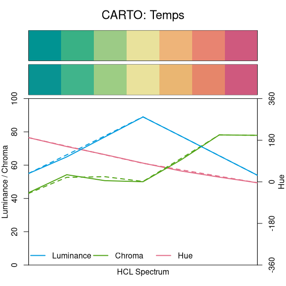
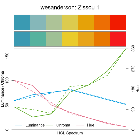
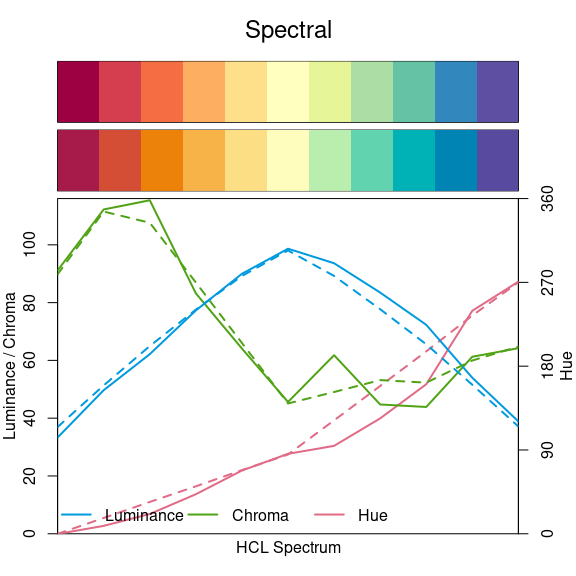
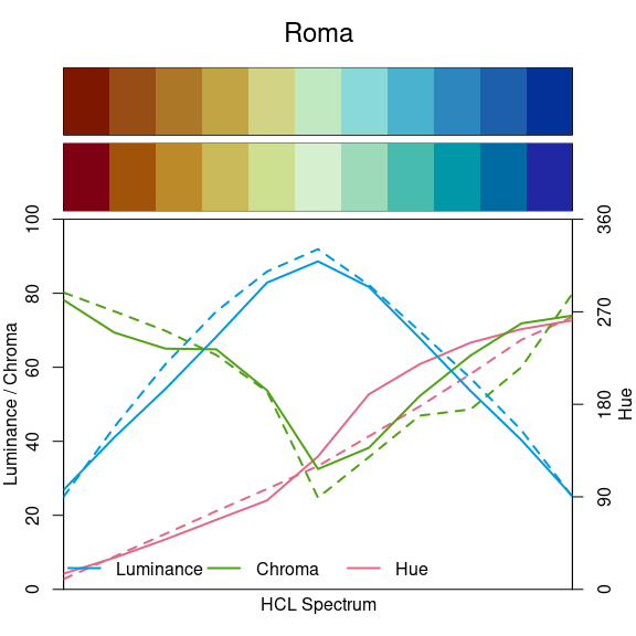
Finally, we compare the flexible diverging “Temps” palette, originally from CARTO, and the “Zissou 1” palette from the wesanderson (Ram and Wickham 2018) package. Both employ a similar hue trajectory going from blue/green via yellow to orange/red. Also, the luminance trajectory is similar but for “Temps” this is more balanced and provides a stronger luminance contrast. The chroma trajectory is rather unbalanced in both palettes but for “Zissou 1” much more so, leading to very high-chroma colors throughout. Thus, both palettes are more suitable for palettes with fewer colors but in “Zissou 1” this issue is more pronounced.