Color Manipulation and Utilities
manipulation_utilities.RmdOverview
The colorspace package provides several color manipulation utilities that are useful for creating, assessing, or transforming color palettes, namely:
-
desaturate(): Desaturate colors by chroma removal in HCL space. -
darken()andlighten(): Algorithmically lighten or darken colors in HCL and/or HLS space. -
adjust_transparency()andextract_transparency(): Adjust or extract the transparency of colors. -
contrast_ratio(): Computing and visualizing W3C contrast ratios of colors. -
max_chroma(): Compute maximum chroma for given hue and luminance in HCL space. -
mixcolor(): Additively mix two colors by computing their convex combination.
Desaturation in HCL space
Desaturation should map a given color to the gray with the same “brightness”. In principle, any perceptually-based color model (HCL, HLS, HSV, …) could be employed for this but HCL works particularly well because its coordinates capture the perceptual properties better than most other color models.
The desaturate() function converts any given hex color
code or named R color to the corresponding HCL coordinates and sets the
chroma to zero. Thus, only the luminance matters which captures the
“brightness” mentioned above. Finally, the resulting HCL coordinates are
transformed back to hex color codes for use in R.
For illustration, a few simple examples are presented below. More examples in the context of palettes for statistical graphics are discussed along with the color vision deficiency article.
First, desaturate() is used to desaturate a vector of R
color names:
desaturate(c("white", "orange", "blue", "black"))## [1] "#FFFFFF" "#B8B8B8" "#4C4C4C" "#000000"Notice that the hex codes corresponding to three coordinates in sRGB space are always the same, indicating gray colors.
Analogously, hex color codes can also be transformed - in this case
RGB rainbow colors from the base R function rainbow():
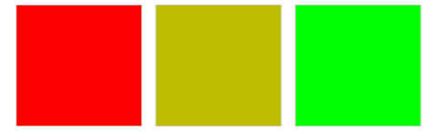
rainbow(3)## [1] "#FF0000" "#00FF00" "#0000FF"
desaturate(rainbow(3))## [1] "#7F7F7F" "#DCDCDC" "#4C4C4C"Even this simple example suffices to show that the three RGB rainbow
colors have very different grayscale levels. This deficiency is even
clearer when using a full color wheel (of colors with hues in [0, 360]
degrees). While the RGB rainbow() is very unbalanced the
HCL rainbow_hcl() (or also qualitative_hcl())
is (by design) balanced with respect to luminance.
wheel <- function(col, radius = 1, ...)
  pie(rep(1, length(col)), col = col, radius = radius, ...)
par(mar = rep(0.5, 4), mfrow = c(2, 2))
wheel(rainbow(8))
wheel(desaturate(rainbow(8)))
wheel(rainbow_hcl(8))
wheel(desaturate(rainbow_hcl(8)))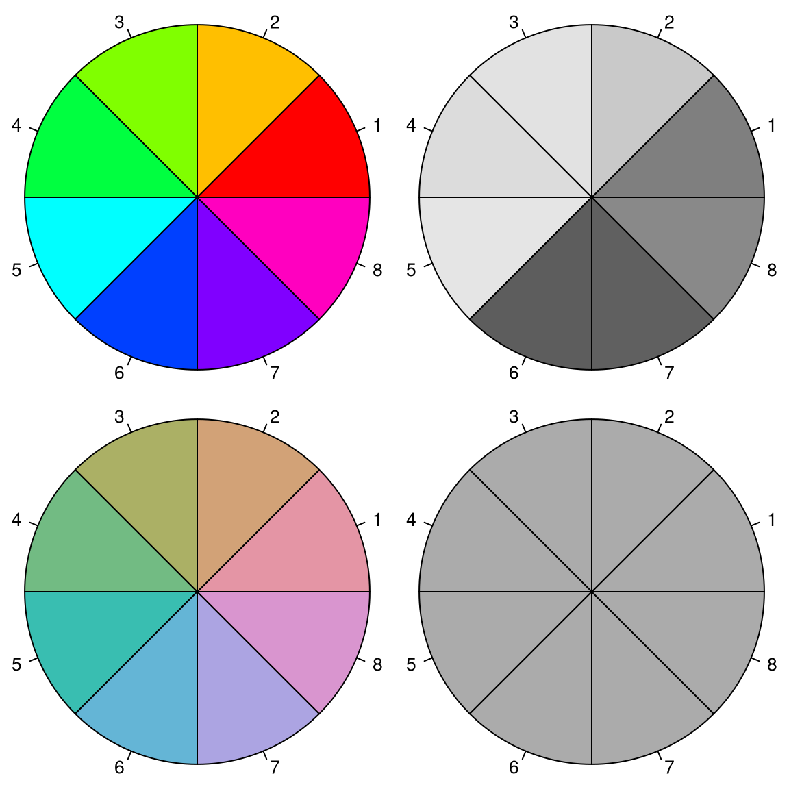
Lighten or darken colors
In principle, a similar approach for lightening and darkening colors can be employed as for desaturation above. The colors can simply be transformed to HCL space and then the luminance can either be decreased (turning the color darker) or increased (turning it lighter) while preserving the hue and chroma coordinates.
This strategy typically works well for lightening colors, although in some situations the result can be rather colorful. Conversely, when darkening rather light colors with little chroma, this can result in rather gray colors.
In these situations, an alternative might be to apply the analogous strategy in HLS space which is frequently used in HTML style sheets. However, this strategy may also yield colors that are either too gray or too colorful. A compromise that sometimes works well is to adjust the luminance coordinate in HCL space but to take the chroma coordinate corresponding to the HLS transformation.
We have found that typically the HCL-based transformation performs
best for lightening colors and this is hence the default in
lighten(). For darkening colors, the combined strategy
often works best and is hence the default in darken(). In
either case it is recommended to try the other available strategies in
case the default yields unexpected results.
Regardless of the chosen color space, the adjustment of the
L component can occur by two methods, relative (the
default) and absolute. For example L - 100 * amount is used
for absolute darkening, or L * (1 - amount) for relative
darkening. See lighten() and darken() for more
details.
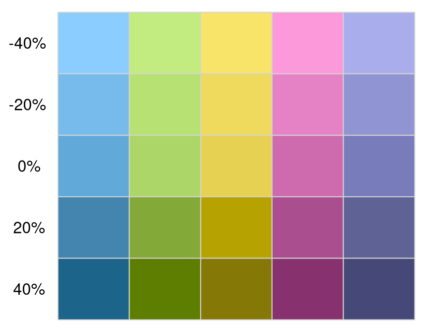
For illustration a qualitative palette (Okabe-Ito) is transformed by two levels of both lightening and darkening, respectively.
oi <- c("#61A9D9", "#ADD668", "#E6D152", "#CE6BAF", "#797CBA")
swatchplot(
  "-40%" = lighten(oi, 0.4),
  "-20%" = lighten(oi, 0.2),
  "  0%" = oi,
  " 20%" =  darken(oi, 0.2),
  " 40%" =  darken(oi, 0.4),
  off = c(0, 0)
)
Adjust or extract the transparency of colors
Alpha transparency is useful for making colors semi-transparent, e.g., for overlaying different elements in graphics. An alpha value (or alpha channel) of 0 (or 00 in hex strings) corresponds to fully transparent and an alpha value of 1 (or FF in hex strings) corresponds to fully opaque. If a color hex string in R does not provide an explicit alpha transparency, the color is assumed to be fully opaque.
The adjust_transparency() function can be used to adjust
the alpha transparency of a set of colors. It always returns a hex color
specification. This hex color can have the alpha transparency
added/removed/modified depending on the specification of the argument
alpha:
-
alpha = NULL: Returns a hex vector with alpha transparency only if needed. Thus, it keeps the alpha transparency for the colors (if any) but only if different from opaque. -
alpha = TRUE: Returns a hex vector with alpha transparency for all colors, using opaque (FF) as the default if missing. -
alpha = FALSE: Returns a hex vector without alpha transparency for all colors (even if the original colors had non-opaque alpha). -
alphanumeric: Returns a hex vector with alpha transparency for all colors set to thealphaargument (recycled if necessary).
For illustration, the transparency of a single black color is
modified to three alpha levels: fully transparent, semi-transparent, and
fully opaque, respectively. Black can be equivalently specified by name
("black"), hex string ("#000000"), or integer
position in the palette (1).
adjust_transparency("black", alpha = c(0, 0.5, 1))## [1] "#00000000" "#00000080" "#000000FF"
adjust_transparency("#000000", alpha = c(0, 0.5, 1))## [1] "#00000000" "#00000080" "#000000FF"
adjust_transparency(1, alpha = c(0, 0.5, 1))## [1] "#00000000" "#00000080" "#000000FF"Subsequently, different settings of alpha are
illustrated for adjusting a vector with three shades of gray, specified
by name (gray, opaque), opaque hex string
("#BEBEBE"), and semi-transparent hex string
("#BEBEBE80"). Four types of adjustment are shown: only if
necessary (alpha = NULL), add (alpha = TRUE),
remove (alpha = FALSE), or modify
(alpha = 0.8).
x <- c("gray", "#BEBEBE", "#BEBEBE80")
adjust_transparency(x, alpha = NULL)
## [1] "#BEBEBE" "#BEBEBE" "#BEBEBE80"
adjust_transparency(x, alpha = TRUE)## [1] "#BEBEBEFF" "#BEBEBEFF" "#BEBEBE80"
adjust_transparency(x, alpha = FALSE)## [1] "#BEBEBE" "#BEBEBE" "#BEBEBE"
adjust_transparency(x, alpha = 0.8)## [1] "#BEBEBECC" "#BEBEBECC" "#BEBEBECC"The extract_transparency() function can be used to
extract the alpha transparency from a set of colors. It allows to
specify the default value - that should be used for colors
without an explicit alpha transparency (defaulting to fully opaque) -
and mode of the return value. This can either be numeric
(in [0, 1]), integer (0L, 1L, …, 255L), character (“00”, “01”, …, “FF”),
or an object of class hexmode (internally represented as
integer with printing as character). The default can use
any of these modes as well (independent of the output mode)
or be NA.
For illustration we extract the transparency from the gray colors in
x in different formats and with different default
values
extract_transparency(x, mode = "numeric")## [1] 1.0000000 1.0000000 0.5019608
extract_transparency(x, mode = "hexmode")## [1] "ff" "ff" "80"
extract_transparency(x, default = NA)## [1] NA NA 0.5019608
extract_transparency(x, default = "80", mode = "integer")## [1] 128 128 128Compute and visualize W3C contrast ratios
The Web Content Accessibility Guidelines (WCAG) by the World Wide Web Consortium (W3C) recommend a contrast ratio of at least 4.5 for the color of regular text on the background color, and a ratio of at least 3 for large text. See . This relies on a specific definition of relative luminances (essentially based on power-transformed sRGB coordinates) that is different from the perceptual luminance as defined, for example, in the HCL color model. Note also that the WCAG pertain to text and background color and not to colors used in data visualization.
For illustration we compute and visualize the contrast ratios of the default palette in R compared to a white background.
contrast_ratio(palette(), "white")## [1] 21.000000 3.758588 1.973030 3.163940 1.603030 4.805641 1.608044
## [8] 2.679156
contrast_ratio(palette(), "white", plot = TRUE)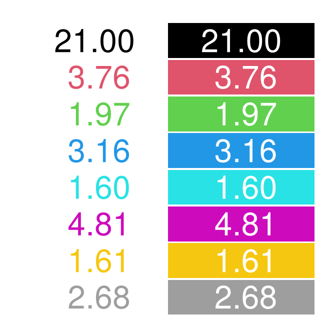
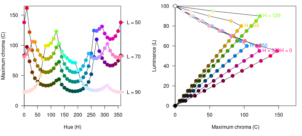
Maximum chroma for given hue and luminance
As the possible combinations of chroma and luminance in HCL space
depend on hue, it is not obvious which trajectories through HCL space
are possible prior to trying a specific HCL coordinate by calling
polarLUV(). To avoid having to fix up the color upon
conversion to RGB hex() color codes, the
max_chroma() function computes (approximately) the maximum
chroma possible.
For illustration we show that for given luminance (here: L = 50) the maximum chroma varies substantially with hue:
max_chroma(h = seq(0, 360, by = 60), l = 50)## [1] 137.96 59.99 69.06 39.81 65.45 119.54 137.96Similarly, maximum chroma also varies substantially across luminance values for a given hue (here: H = 120, green):
max_chroma(h = 120, l = seq(0, 100, by = 20))## [1] 0.00 28.04 55.35 82.79 110.28 0.00In the plots below more combinations are visualized: In the left panel for maximum chroma across hues given luminance and in the right panel with increasing luminance given hue.